Demo MAGxHR_1B (magnetic field 50Hz)
Authors: Ashley Smith
Abstract: Access to the high rate (50Hz) magnetic data (level 1b product).
%load_ext watermark
%watermark -i -v -p viresclient,pandas,xarray,matplotlib
2021-01-24T15:45:34+00:00

CPython 3.7.6
IPython 7.11.1

viresclient 0.7.1
pandas 0.25.3
xarray 0.15.0
matplotlib 3.1.2
from viresclient import SwarmRequest
import datetime as dt
import matplotlib.pyplot as plt
request = SwarmRequest()
MAGX_HR_1B product information
The 50Hz measurements of the magnetic field vector (B_NEC) and total intensity (F).
Documentation:
https://earth.esa.int/web/guest/missions/esa-eo-missions/swarm/data-handbook/level-1b-product-definitions#MAGX_HR_1B_Product
Measurements are available through VirES as part of collections with names containing MAGx_HR, for each Swarm spacecraft:
request.available_collections("MAG_HR", details=False)
{'MAG_HR': ['SW_OPER_MAGA_HR_1B', 'SW_OPER_MAGB_HR_1B', 'SW_OPER_MAGC_HR_1B']}
The measurements can be used together with geomagnetic model evaluations as shall be shown below.
Check what “MAG” data variables are available
request.available_measurements("MAG_HR")
['F',
 'B_VFM',
 'B_NEC',
 'dB_Sun',
 'dB_AOCS',
 'dB_other',
 'B_error',
 'q_NEC_CRF',
 'Att_error',
 'Flags_B',
 'Flags_q',
 'Flags_Platform']
Fetch data
request = SwarmRequest()
request.set_collection("SW_OPER_MAGA_HR_1B")
request.set_products(
   measurements=request.PRODUCT_VARIABLES['MAG_HR'],
   sampling_step="PT0.019S", # ~50Hz sampling
)
data = request.get_between(
   start_time="2015-06-21T12:00:00Z",
   end_time="2015-06-21T12:01:00Z",
   asynchronous=False
)
Downloading: 100%|██████████| [ Elapsed: 00:00, Remaining: 00:00 ] (0.714MB)
data.sources
['SW_OPER_MAGA_HR_1B_20150621T000000_20150621T235959_0505_MDR_MAG_HR']
ds = data.as_xarray()
ds
<xarray.Dataset>
Dimensions:         (NEC: 3, Timestamp: 3000, VFM: 3, quaternion: 4)
Coordinates:
  * Timestamp       (Timestamp) datetime64[ns] 2015-06-21T12:00:00.007250071 ... 2015-06-21T12:00:59.983929634
  * NEC             (NEC) <U1 'N' 'E' 'C'
  * VFM             (VFM) <U1 'i' 'j' 'k'
  * quaternion      (quaternion) <U1 '1' 'i' 'j' 'k'
Data variables:
    Spacecraft      (Timestamp) object 'A' 'A' 'A' 'A' 'A' ... 'A' 'A' 'A' 'A'
    Longitude       (Timestamp) float64 -17.17 -17.17 -17.17 ... -17.12 -17.12
    Latitude        (Timestamp) float64 -41.84 -41.83 -41.83 ... -38.01 -38.01
    dB_Sun          (Timestamp, VFM) float64 0.7188 -0.6263 ... -0.4607 -0.0792
    Att_error       (Timestamp) float64 1.365 1.365 1.365 ... 1.138 1.137 1.136
    B_error         (Timestamp, VFM) float64 0.2217 0.2219 ... 0.2167 0.4135
    Flags_B         (Timestamp) uint8 0 0 0 0 0 0 0 0 0 0 ... 0 0 0 0 0 0 0 0 0
    Radius          (Timestamp) float64 6.837e+06 6.837e+06 ... 6.836e+06
    dB_other        (Timestamp, VFM) float64 0.0349 0.0184 ... 0.019 -0.0463
    q_NEC_CRF       (Timestamp, quaternion) float64 0.0006543 -0.006776 ... -1.0
    Flags_q         (Timestamp) uint8 0 0 0 0 0 0 0 0 0 0 ... 0 0 0 0 0 0 0 0 0
    B_NEC           (Timestamp, NEC) float64 9.677e+03 -3.495e+03 ... -1.817e+04
    F               (Timestamp) float64 2.109e+04 2.109e+04 ... 2.087e+04
    Flags_Platform  (Timestamp) uint16 1 1 1 1 1 1 1 1 1 1 ... 1 1 1 1 1 1 1 1 1
    B_VFM           (Timestamp, VFM) float64 -1.562e+04 -4.153e+03 ... -1.34e+04
    dB_AOCS         (Timestamp, VFM) float64 0.1054 -0.2643 ... -0.1057 -4.884
Attributes:
    Sources:         ['SW_OPER_MAGA_HR_1B_20150621T000000_20150621T235959_050...
    MagneticModels:  []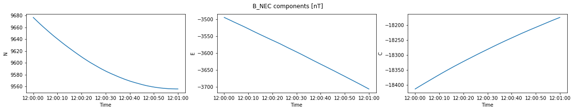
RangeFilters: []fig, axes = plt.subplots(figsize=(20, 3), ncols=3, sharex=True)
for i in range(3):
axes[i].plot(ds["Timestamp"], ds["B_NEC"][:, i])
axes[i].set_ylabel("NEC"[i])
axes[i].set_xlabel("Time")
fig.suptitle("B_NEC components [nT]");
/opt/conda/lib/python3.7/site-packages/pandas/plotting/_matplotlib/converter.py:103: FutureWarning: Using an implicitly registered datetime converter for a matplotlib plotting method. The converter was registered by pandas on import. Future versions of pandas will require you to explicitly register matplotlib converters.

To register the converters:
	>>> from pandas.plotting import register_matplotlib_converters
	>>> register_matplotlib_converters()
  warnings.warn(msg, FutureWarning)
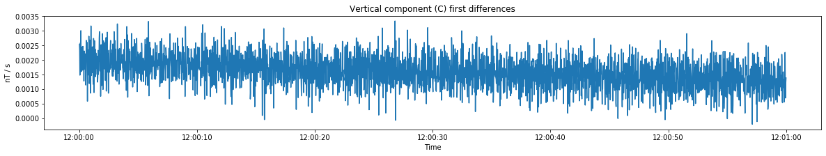
import numpy as np

fig, ax = plt.subplots(figsize=(20, 3))
dBdt = np.diff(ds["B_NEC"], axis=0) * (1/50)
ax.plot(ds["Timestamp"][1:], dBdt[:, 2])
ax.set_ylabel("nT / s")
ax.set_xlabel("Time")
ax.set_title("Vertical component (C) first differences");