Demo TECxTMS_2F (total electron content)
Authors: Ashley Smith
Abstract: Access to the total electric contents (level 2 product).
%load_ext watermark
%watermark -i -v -p viresclient,pandas,xarray,matplotlib
2021-01-24T15:45:59+00:00

CPython 3.7.6
IPython 7.11.1

viresclient 0.7.1
pandas 0.25.3
xarray 0.15.0
matplotlib 3.1.2
from viresclient import SwarmRequest
import datetime as dt
import numpy as np
import pandas as pd
import matplotlib.pyplot as plt

request = SwarmRequest()
TECxTMS_2F product information
Derived total electron content (TEC)
Documentation:
https://earth.esa.int/web/guest/missions/esa-eo-missions/swarm/data-handbook/level-2-product-definitions#TECxTMS_2F
Check what “TEC” data variables are available
request.available_collections("IPD", details=False)
{'IPD': ['SW_OPER_IPDAIRR_2F', 'SW_OPER_IPDBIRR_2F', 'SW_OPER_IPDCIRR_2F']}
request.available_measurements("TEC")
['GPS_Position',
 'LEO_Position',
 'PRN',
 'L1',
 'L2',
 'P1',
 'P2',
 'S1',
 'S2',
 'Elevation_Angle',
 'Absolute_VTEC',
 'Absolute_STEC',
 'Relative_STEC',
 'Relative_STEC_RMS',
 'DCB',
 'DCB_Error']
Fetch one day of TEC data
request.set_collection("SW_OPER_TECATMS_2F")
request.set_products(measurements=request.available_measurements("TEC"))
data = request.get_between(dt.datetime(2014,1,1),
                           dt.datetime(2014,1,2))
[1/1] Processing:  100%|██████████|  [ Elapsed: 00:01, Remaining: 00:00 ]
      Downloading: 100%|██████████|  [ Elapsed: 00:00, Remaining: 00:00 ] (9.311MB)
Loading as pandas
df = data.as_dataframe()
df.head()
| DCB_Error | Elevation_Angle | S2 | DCB | Relative_STEC_RMS | Spacecraft | Latitude | L1 | PRN | Absolute_VTEC | P2 | Radius | LEO_Position | Longitude | Absolute_STEC | L2 | P1 | GPS_Position | S1 | Relative_STEC | |
|---|---|---|---|---|---|---|---|---|---|---|---|---|---|---|---|---|---|---|---|---|
| Timestamp | ||||||||||||||||||||
| 2014-01-01 00:00:04 | 0.832346 | 39.683333 | 36.83 | -11.446853 | 0.555675 | A | -1.482419 | -6.261986e+06 | 15 | 10.894886 | 2.182914e+07 | 6.878338e+06 | [6668214.544000001, -1677732.674, -177943.9959... | -14.122572 | 16.429938 | -6.261989e+06 | 2.182913e+07 | [22448765.690377887, 5421379.431197803, -13409... | 36.83 | 24.041127 |
| 2014-01-01 00:00:04 | 0.832346 | 37.478137 | 34.75 | -11.446853 | 0.488000 | A | -1.482419 | -1.466568e+07 | 18 | 10.461554 | 2.135749e+07 | 6.878338e+06 | [6668214.544000001, -1677732.674, -177943.9959... | -14.122572 | 16.456409 | -1.466568e+07 | 2.135749e+07 | [16113499.491062254, -16306172.004347403, -126... | 34.75 | 22.754795 |
| 2014-01-01 00:00:04 | 0.832346 | 24.681787 | 30.90 | -11.446853 | 1.313984 | A | -1.482419 | -5.455452e+06 | 22 | 9.529846 | 2.277638e+07 | 6.878338e+06 | [6668214.544000001, -1677732.674, -177943.9959... | -14.122572 | 20.434286 | -5.455454e+06 | 2.277638e+07 | [10823457.339250825, -24014739.352816023, -248... | 30.90 | 15.585271 |
| 2014-01-01 00:00:04 | 0.832346 | 24.647445 | 29.87 | -11.446853 | 0.899036 | A | -1.482419 | -3.402816e+06 | 24 | 9.357587 | 2.298847e+07 | 6.878338e+06 | [6668214.544000001, -1677732.674, -177943.9959... | -14.122572 | 20.085094 | -3.402821e+06 | 2.298846e+07 | [20631539.59055339, 13441368.439225309, 100505... | 29.87 | 52.291341 |
| 2014-01-01 00:00:04 | 0.832346 | 30.753636 | 30.88 | -11.446853 | 0.546729 | A | -1.482419 | -2.285981e+06 | 25 | 8.597559 | 2.229900e+07 | 6.878338e+06 | [6668214.544000001, -1677732.674, -177943.9959... | -14.122572 | 15.676947 | -2.285986e+06 | 2.229899e+07 | [16637723.905075422, -10692759.977004562, 1761... | 30.88 | 52.672067 |
NB: The time interval is not always the same:
times = df.index
np.unique(np.sort(np.diff(times.to_pydatetime())))
array([datetime.timedelta(0), datetime.timedelta(seconds=10)],
      dtype=object)
len(df), 60*60*24
(49738, 86400)
Loading and plotting as xarray
ds = data.as_xarray()
ds
<xarray.Dataset>
Dimensions:            (Timestamp: 49738, WGS84: 3)
Coordinates:
  * Timestamp          (Timestamp) datetime64[ns] 2014-01-01T00:00:04 ... 2014-01-01T23:59:54
  * WGS84              (WGS84) <U1 'X' 'Y' 'Z'
Data variables:
    Spacecraft         (Timestamp) object 'A' 'A' 'A' 'A' ... 'A' 'A' 'A' 'A'
    Elevation_Angle    (Timestamp) float64 39.68 37.48 24.68 ... 49.64 45.71
    S2                 (Timestamp) float64 36.83 34.75 30.9 ... 23.03 37.73 37.5
    Relative_STEC_RMS  (Timestamp) float64 0.5557 0.488 1.314 ... 0.6458 3.041
    Latitude           (Timestamp) float64 -1.482 -1.482 -1.482 ... -81.7 -81.7
    Absolute_VTEC      (Timestamp) float64 10.89 10.46 9.53 ... 8.365 7.912
    P2                 (Timestamp) float64 2.183e+07 2.136e+07 ... 2.171e+07
    S1                 (Timestamp) float64 36.83 34.75 30.9 ... 23.03 37.73 37.5
    Relative_STEC      (Timestamp) float64 24.04 22.75 15.59 ... 16.92 26.51
    DCB_Error          (Timestamp) float64 0.8323 0.8323 ... 0.8323 0.8323
    DCB                (Timestamp) float64 -11.45 -11.45 ... -11.45 -11.45
    L1                 (Timestamp) float64 -6.262e+06 -1.467e+07 ... -3.41e+06
    PRN                (Timestamp) uint16 15 18 22 24 25 29 ... 7 15 16 18 21 26
    Radius             (Timestamp) float64 6.878e+06 6.878e+06 ... 6.88e+06
    LEO_Position       (Timestamp, WGS84) float64 6.668e+06 ... -6.808e+06
    Longitude          (Timestamp) float64 -14.12 -14.12 -14.12 ... 1.559 1.559
    Absolute_STEC      (Timestamp) float64 16.43 16.46 20.43 ... 10.77 10.78
    L2                 (Timestamp) float64 -6.262e+06 -1.467e+07 ... -3.41e+06
    P1                 (Timestamp) float64 2.183e+07 2.136e+07 ... 2.171e+07
    GPS_Position       (Timestamp, WGS84) float64 2.245e+07 ... -2.111e+07
Attributes:
    Sources:         ['SW_OPER_TECATMS_2F_20140101T000000_20140101T235959_0301']
    MagneticModels:  []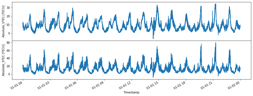
RangeFilters: []fig, axes = plt.subplots(nrows=2, ncols=1, figsize=(15,5), sharex=True)
ds["Absolute_VTEC"].plot.line(x="Timestamp", ax=axes[0])
ds["Absolute_STEC"].plot.line(x="Timestamp", ax=axes[1]);
fig.subplots_adjust(hspace=0)
/opt/conda/lib/python3.7/site-packages/pandas/plotting/_matplotlib/converter.py:103: FutureWarning: Using an implicitly registered datetime converter for a matplotlib plotting method. The converter was registered by pandas on import. Future versions of pandas will require you to explicitly register matplotlib converters.

To register the converters:
	>>> from pandas.plotting import register_matplotlib_converters
	>>> register_matplotlib_converters()
  warnings.warn(msg, FutureWarning)