Demo FACxTMS_2F (single satellite)
Authors: Ashley Smith
Abstract: Access to the field aligned currents evaluated by the single satellite method (level 2 product). We show simple line plots of the time series over short periods (minutes), from both Swarm Alpha and Charlie. We also compare with the alternative method whereby the FACs are evaluated locally by computing them from the magnetic field data (
B_NECfromMAGx_LR_1B).
Documentation:
https://earth.esa.int/web/guest/missions/esa-eo-missions/swarm/data-handbook/level-2-product-definitions#FACxTMS_2F
https://earth.esa.int/documents/10174/1514862/Swarm_L2_FAC_single_product_description
%load_ext watermark
%watermark -i -v -p viresclient,pandas,xarray,matplotlib
2021-01-24T15:46:05+00:00

CPython 3.7.6
IPython 7.11.1

viresclient 0.7.1
pandas 0.25.3
xarray 0.15.0
matplotlib 3.1.2
from viresclient import SwarmRequest
import datetime as dt
import numpy as np
import pandas as pd
import matplotlib.pyplot as plt
import matplotlib.dates as mdates
import cartopy.crs as ccrs
import cartopy.feature as cfeature

request = SwarmRequest()
Check what “FAC” data variables are available
NB: these are the same as in the FAC_TMS_2F dual-satellite FAC product
request.available_collections("FAC", details=False)
{'FAC': ['SW_OPER_FACATMS_2F',
  'SW_OPER_FACBTMS_2F',
  'SW_OPER_FACCTMS_2F',
  'SW_OPER_FAC_TMS_2F']}
request.available_measurements("FAC")
['IRC',
 'IRC_Error',
 'FAC',
 'FAC_Error',
 'Flags',
 'Flags_F',
 'Flags_B',
 'Flags_q']
Plotting as a time series
Fetch one day from Swarm Alpha and Charlie
Also fetch the quasidipole (QD) coordinates and Orbit Number at the same time.
request.set_collection("SW_OPER_FACATMS_2F", "SW_OPER_FACCTMS_2F")
request.set_products(
    measurements=["FAC", "FAC_Error",
                  "Flags", "Flags_F", "Flags_B", "Flags_q"],
    auxiliaries=["QDLat", "QDLon", "OrbitNumber"],
)
data = request.get_between(
    dt.datetime(2014,4,20),
    dt.datetime(2014,4,21)
)
[1/1] Processing:  100%|██████████|  [ Elapsed: 00:01, Remaining: 00:00 ]
      Downloading: 100%|██████████|  [ Elapsed: 00:00, Remaining: 00:00 ] (14.696MB)
The source files of the original data are listed
data.sources
['SW_OPER_AUXAORBCNT_20131122T000000_20210124T000000_0001',
 'SW_OPER_AUXCORBCNT_20131122T000000_20210124T000000_0001',
 'SW_OPER_FACATMS_2F_20140420T000000_20140420T235959_0301',
 'SW_OPER_FACCTMS_2F_20140420T000000_20140420T235959_0301']
The data can be loaded as a pandas dataframe
df = data.as_dataframe()
df.head()
| OrbitNumber | Flags | Spacecraft | Flags_B | Longitude | Flags_F | QDLon | Latitude | Flags_q | QDLat | Radius | FAC | FAC_Error | |
|---|---|---|---|---|---|---|---|---|---|---|---|---|---|
| Timestamp | |||||||||||||
| 2014-04-20 00:00:00.500 | 2267 | 0 | A | 0 | 19.102806 | 2 | 87.677834 | -26.849183 | 0 | -36.222496 | 6851357.065 | 0.005852 | 0.065746 |
| 2014-04-20 00:00:01.500 | 2267 | 0 | A | 0 | 19.102319 | 2 | 87.701988 | -26.785503 | 0 | -36.172024 | 6851350.555 | 0.008188 | 0.066112 |
| 2014-04-20 00:00:02.500 | 2267 | 0 | A | 0 | 19.101828 | 2 | 87.726082 | -26.721823 | 0 | -36.121502 | 6851344.035 | 0.012294 | 0.066744 |
| 2014-04-20 00:00:03.500 | 2267 | 0 | A | 0 | 19.101333 | 2 | 87.750122 | -26.658143 | 0 | -36.070930 | 6851337.505 | 0.002132 | 0.065236 |
| 2014-04-20 00:00:04.500 | 2267 | 0 | A | 0 | 19.100834 | 2 | 87.774101 | -26.594462 | 0 | -36.020313 | 6851330.965 | -0.001669 | 0.064682 |
Alternatively we can load the data as an xarray Dataset, though in the following examples we use the data via a pandas DataFrame instead
ds = data.as_xarray()
ds
<xarray.Dataset>
Dimensions:      (Timestamp: 172800)
Coordinates:
  * Timestamp    (Timestamp) datetime64[ns] 2014-04-20T00:00:00.500000 ... 2014-04-20T23:59:59.500000
Data variables:
    Spacecraft   (Timestamp) object 'A' 'A' 'A' 'A' 'A' ... 'C' 'C' 'C' 'C' 'C'
    OrbitNumber  (Timestamp) int32 2267 2267 2267 2267 ... 2279 2279 2279 2279
    Flags        (Timestamp) uint32 0 0 0 0 0 0 0 0 0 0 ... 0 0 0 0 0 0 0 0 0 0
    Flags_B      (Timestamp) uint32 0 0 0 0 0 0 0 0 0 0 ... 0 0 0 0 0 0 0 0 0 0
    Longitude    (Timestamp) float64 19.1 19.1 19.1 19.1 ... 100.6 102.0 103.3
    Flags_F      (Timestamp) uint32 2 2 2 2 2 2 2 2 2 2 ... 2 2 2 2 2 2 2 2 2 2
    QDLon        (Timestamp) float64 87.68 87.7 87.73 ... 171.9 172.4 172.8
    Latitude     (Timestamp) float64 -26.85 -26.79 -26.72 ... 87.31 87.33 87.33
    Flags_q      (Timestamp) uint32 0 0 0 0 0 ... 20020 20020 20020 20020 20020
    QDLat        (Timestamp) float64 -36.22 -36.17 -36.12 ... 81.26 81.27 81.28
    Radius       (Timestamp) float64 6.851e+06 6.851e+06 ... 6.835e+06 6.835e+06
    FAC          (Timestamp) float64 0.005852 0.008188 ... 0.08035 0.005977
    FAC_Error    (Timestamp) float64 0.06575 0.06611 0.06674 ... 0.0453 0.05645
Attributes:
    Sources:         ['SW_OPER_AUXAORBCNT_20131122T000000_20210124T000000_000...
    MagneticModels:  []
    RangeFilters:    []
Depending on your application, you should probably do some filtering according to each of the flags. This can be done on the dataframe here, or beforehand on the server using request.set_range_filter(). See https://earth.esa.int/documents/10174/1514862/Swarm_L2_FAC_single_product_description for more about the data
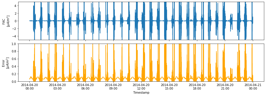
Plot the time series (FAC and FAC_Error for Alpha)
fig, axes = plt.subplots(ncols=1, nrows=2, figsize=(15,5))
# Select out the time series from Swarm Alpha
dfA = df.where(df["Spacecraft"] == "A").dropna()
axes[0].plot(dfA.index, dfA["FAC"])
axes[1].plot(dfA.index, dfA["FAC_Error"], color="orange")
axes[0].set_ylabel("FAC\n[$\mu A / m^2$]");
axes[1].set_ylabel("Error\n[$\mu A / m^2$]");
axes[1].set_xlabel("Timestamp");
date_format = mdates.DateFormatter('%Y-%m-%d\n%H:%M')
axes[1].xaxis.set_major_formatter(date_format)
axes[0].set_ylim(-5, 5);
axes[1].set_ylim(0, 1);
axes[0].set_xticklabels([])
fig.subplots_adjust(hspace=0.1)
/opt/conda/lib/python3.7/site-packages/pandas/plotting/_matplotlib/converter.py:103: FutureWarning: Using an implicitly registered datetime converter for a matplotlib plotting method. The converter was registered by pandas on import. Future versions of pandas will require you to explicitly register matplotlib converters.

To register the converters:
	>>> from pandas.plotting import register_matplotlib_converters
	>>> register_matplotlib_converters()
  warnings.warn(msg, FutureWarning)
Plot a subset of the time series (FAC from Alpha and Charlie)
def line_plot(fig, ax, df, varname="FAC", spacecraft="A", color="red"):
    """Plot FAC as a line, given a dataframe"""
    df = df.copy()
    df = df.where(df["Spacecraft"] == spacecraft).dropna()
    ax.plot(df.index, df[varname], linewidth=1,
            label=f"{varname}$_{spacecraft}$", color=color)
    # Plot error range as filled area
    if varname is "FAC":
        ax.fill_between(df.index,
                        df["FAC"] - df["FAC_Error"],
                        df["FAC"] + df["FAC_Error"], color="grey")
    # Adjust limits and label formatting
    datetime_format = "%Y-%m-%d\n%H:%M:%S"
    xlabel_format = mdates.DateFormatter(datetime_format)
    ax.xaxis.set_major_formatter(xlabel_format)
    ax.set_ylabel("[ $\mu A / m^2$ ]")
    # Make y-axis symmetric about zero
    ylim = max(abs(y) for y in ax.get_ylim())
    ax.set_ylim((-ylim, ylim))
    ax.legend()
    ax.grid(True)
    # Set up an extra xaxis at the top, to display Latitude
    ax2 = ax.twiny()
    ax2.set_xlim(ax.get_xlim())
    ax2.set_xticks(ax.get_xticks())
    # Identify closest times in dataframe to use for Latitude labels
    # NB need to draw the figure now in order to get the xticklabels
    #  https://stackoverflow.com/a/41124884
    fig.canvas.draw()
    # Extract times from the lower x axis
    # Use them to find the nearest Lat values in the dataframe
    xtick_times = [dt.datetime.strptime(ts.get_text(), datetime_format) for ts in ax.get_xticklabels()]
    ilocs = [df.index.get_loc(t, method="nearest") for t in xtick_times]
    lats = df.iloc[ilocs]["Latitude"]
    lat_labels = ["{}°".format(s) for s in np.round(lats.values, decimals=1)]
    ax2.set_xticklabels(lat_labels)
    ax2.set_xlabel("Latitude")

# Easy pandas-style slicing of the dataframe
df_subset = df['2014-04-20T04:26:00':'2014-04-20T04:30:00']
fig, axes = plt.subplots(nrows=2, figsize=(15, 5))
line_plot(fig, axes[0], df_subset, spacecraft="A", color="red")
line_plot(fig, axes[1], df_subset, spacecraft="C", color="blue")
fig.subplots_adjust(hspace=0.8)
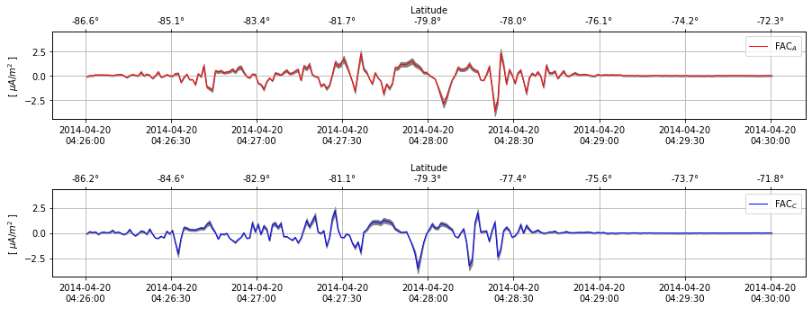
FAC estimates from (top) Swarm Alpha and (bottom) Swarm Charlie. The error estimate is shown as a thin grey area
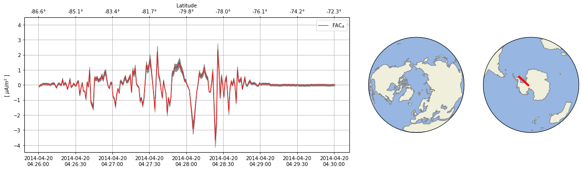
Also show satellite location on a map
def line_plot_figure(df, spacecraft="A", color="red"):
    """Generate a figure containing both line plot and maps"""
    df = df.copy()
    df = df.where(df["Spacecraft"] == spacecraft).dropna()
    # Set up figure geometry together with North/South maps
    fig = plt.figure(figsize=(20, 5))
    ax_lineplot = plt.subplot2grid((1, 5), (0, 0), colspan=3, fig=fig)
    ax_N = plt.subplot2grid((1, 5), (0, 3), fig=fig,
        projection=ccrs.Orthographic(
            central_longitude=0.0, central_latitude=90.0
        ))
    ax_S = plt.subplot2grid((1, 5), (0, 4), fig=fig,
        projection=ccrs.Orthographic(
            central_longitude=0.0, central_latitude=-90.0
        ))
    for _ax in (ax_N, ax_S):
        _ax.set_global()
        _ax.coastlines(color="grey")
        _ax.add_feature(cfeature.LAND)
        _ax.add_feature(cfeature.OCEAN)
        _ax.plot(df["Longitude"], df["Latitude"], transform=ccrs.PlateCarree(),
                 linewidth=4, color=color)
    # Draw the line plot as before
    line_plot(fig, ax_lineplot, df, spacecraft=spacecraft, color=color)

line_plot_figure(df_subset, spacecraft="A", color="red")
/opt/conda/lib/python3.7/site-packages/cartopy/io/__init__.py:260: DownloadWarning: Downloading: http://naciscdn.org/naturalearth/110m/physical/ne_110m_land.zip
  warnings.warn('Downloading: {}'.format(url), DownloadWarning)
/opt/conda/lib/python3.7/site-packages/cartopy/io/__init__.py:260: DownloadWarning: Downloading: http://naciscdn.org/naturalearth/110m/physical/ne_110m_ocean.zip
  warnings.warn('Downloading: {}'.format(url), DownloadWarning)
/opt/conda/lib/python3.7/site-packages/cartopy/io/__init__.py:260: DownloadWarning: Downloading: http://naciscdn.org/naturalearth/110m/physical/ne_110m_coastline.zip
  warnings.warn('Downloading: {}'.format(url), DownloadWarning)
Comparing to values calculated locally from the B_NEC data (experimental)
ref https://nbviewer.jupyter.org/github/smithara/viresclient_examples/blob/master/swarmpyfac_dev.ipynb
NB this is currently fixed to the time window and satellite combination (A and C) set above
from swarmpyfac.fac import single_sat_fac

def _fetch_data(start='2014-04-20T04:26:00',
                end='2014-04-20T04:30:02', spacecraft="A"):
    """Fetch B_NEC data and combined geomagnetic model for a given spacecraft"""
    request = SwarmRequest()
    request.set_collection(f"SW_OPER_MAG{spacecraft}_LR_1B")
    request.set_products(
        measurements=["B_NEC"],
        models=['Model = "MCO_SHA_2C" + "MLI_SHA_2C" + "MMA_SHA_2C-Primary" + "MMA_SHA_2C-Secondary"'])
    data = request.get_between(start, end,
                             asynchronous=False, show_progress=False)
    return data.as_xarray()

def _get_input_data_from_ds(ds):
    """Extract the "input_data" required from the dataset"""
    # convert time to unix time seconds
    ## if on a dataframe, df:
    ## time = np.array(df.index.astype(np.int64) / 10**9)
    # on xarray.Dataset:
    time = ds['Timestamp'].data.astype(np.int64) / 10**9
    theta = ds['Latitude'].data
    phi = ds['Longitude'].data
    r = ds['Radius'].data
    # equivalent to swarmpyfac.utils.pack_3d:
    positions = np.stack((theta, phi, r), axis=1)
    B_model = ds['B_NEC_Model'].data
    B_res = ds['B_NEC'].data - B_model
    return {'time': time, 'positions':positions,
            'B_res': B_res, 'B_model': B_model}

def _append_fac(ds=None):
    """Append FAC calculations to a dataset"""
    input_data = _get_input_data_from_ds(ds)
    output = single_sat_fac(**input_data)
    # outputs like these should probably be turned into a dict so that they can be identified
    irc = output[2]
    fac = output[3]
    time = output[0]
    # Append the new data to the dataset
    # https://xarray.pydata.org/en/stable/data-structures.html#dictionary-like-methods
    # Note that there must now be a new offset time coordinate
    ds.coords['Timestamp_2'] = pd.to_datetime(time, unit='s')
    ds[f'FAC_calculated'] = (('Timestamp_2',), fac)
    ds[f'IRC_calculated'] = (('Timestamp_2',), irc)
    return ds

def append_FAC_calculated_locally(df):
    """Use the functions above to evaluate FAC

    NB currently depends on the fixed time and spacecraft selection as before

    """
    # Create xarray datasets containing the FAC estimates from each of A and C
    ds_A = _append_fac(_fetch_data('2014-04-20T04:26:00',
                                 '2014-04-20T04:30:02', spacecraft="A"))
    ds_C = _append_fac(_fetch_data('2014-04-20T04:26:00',
                                 '2014-04-20T04:30:02', spacecraft="C"))
    # Transform them into a concatenated dataframe
    df_A = pd.DataFrame(ds_A["FAC_calculated"].to_pandas(), columns=["FAC_calc"])
    df_C = pd.DataFrame(ds_C["FAC_calculated"].to_pandas(), columns=["FAC_calc"])
    df_calc = pd.concat((df_A, df_C))
    df_calc.index.name = ""
    # Append them to the existing dataframe
    df = df.copy()
    df["FAC_new"] = df_calc["FAC_calc"]
    return df
Evaluate FACs locally and append to the dataframe
df_subset = append_FAC_calculated_locally(df_subset)
df_subset["FAC_diff"] = df_subset["FAC"] - df_subset["FAC_new"]
df_subset.head()
| OrbitNumber | Flags | Spacecraft | Flags_B | Longitude | Flags_F | QDLon | Latitude | Flags_q | QDLat | Radius | FAC | FAC_Error | FAC_new | FAC_diff | |
|---|---|---|---|---|---|---|---|---|---|---|---|---|---|---|---|
| Timestamp | |||||||||||||||
| 2014-04-20 04:26:00.500 | 2270 | 0 | A | 0 | -96.717204 | 2 | 9.937644 | -86.569620 | 0 | -72.136772 | 6853867.625 | -0.101983 | 0.044831 | -0.100295 | -0.001689 |
| 2014-04-20 04:26:01.500 | 2270 | 0 | A | 0 | -95.910658 | 2 | 9.987845 | -86.528758 | 0 | -72.077850 | 6853868.130 | 0.007275 | 0.061232 | 0.008985 | -0.001710 |
| 2014-04-20 04:26:02.500 | 2270 | 0 | A | 0 | -95.123108 | 2 | 10.037619 | -86.487219 | 0 | -72.018929 | 6853868.625 | -0.004518 | 0.059475 | -0.002786 | -0.001732 |
| 2014-04-20 04:26:03.500 | 2270 | 0 | A | 0 | -94.354184 | 2 | 10.086978 | -86.445027 | 0 | -71.960007 | 6853869.120 | 0.072944 | 0.071107 | 0.074697 | -0.001753 |
| 2014-04-20 04:26:04.500 | 2270 | 0 | A | 0 | -93.603506 | 2 | 10.135930 | -86.402204 | 0 | -71.901085 | 6853869.610 | 0.057414 | 0.068790 | 0.059188 | -0.001774 |
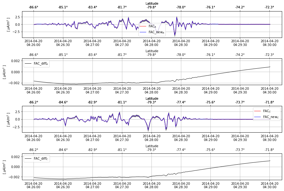
Plot the difference between the FAC sourced from the product, and the one evaluated locally
fig, axes = plt.subplots(nrows=4, figsize=(15, 10))
line_plot(fig, axes[0], df_subset, varname="FAC", spacecraft="A", color="red")
line_plot(fig, axes[0], df_subset, varname="FAC_new", spacecraft="A", color="blue")
line_plot(fig, axes[1], df_subset, varname="FAC_diff", spacecraft="A", color="black")
line_plot(fig, axes[2], df_subset, varname="FAC", spacecraft="C", color="red")
line_plot(fig, axes[2], df_subset, varname="FAC_new", spacecraft="C", color="blue")
line_plot(fig, axes[3], df_subset, varname="FAC_diff", spacecraft="C", color="black")
fig.subplots_adjust(hspace=0.8)