Demo EEFxTMS_2F (equatorial electric field)
Authors: Ashley Smith
Abstract: Access to the equatorial electric field (level 2 product).
%load_ext watermark
%watermark -i -v -p viresclient,pandas,xarray,matplotlib
2021-01-24T15:47:30+00:00

CPython 3.7.6
IPython 7.11.1

viresclient 0.7.1
pandas 0.25.3
xarray 0.15.0
matplotlib 3.1.2
from viresclient import SwarmRequest
import datetime as dt
import numpy as np
import matplotlib.pyplot as plt

request = SwarmRequest()
EEFxTMS_2F product information
Dayside equatorial electric field, sampled at every dayside equator crossing +- 20mins
Documentation:
https://earth.esa.int/web/guest/missions/esa-eo-missions/swarm/data-handbook/level-2-product-definitions#EEFxTMS_2F
Check what “EEF” data variables are available
request.available_collections("EEF", details=False)
{'EEF': ['SW_OPER_EEFATMS_2F', 'SW_OPER_EEFBTMS_2F', 'SW_OPER_EEFCTMS_2F']}
request.available_measurements("EEF")
['EEF', 'EEJ', 'RelErr', 'Flags']
Fetch all the EEF and EEJ values from Bravo during 2016
request.set_collection("SW_OPER_EEFBTMS_2F")
request.set_products(measurements=["EEF", "EEJ", "Flags"])
data = request.get_between(
    dt.datetime(2016,1,1),
    dt.datetime(2017,1,1)
)
[1/1] Processing:  100%|██████████|  [ Elapsed: 00:03, Remaining: 00:00 ]
      Downloading: 100%|██████████|  [ Elapsed: 00:00, Remaining: 00:00 ] (3.834MB)
# The first three and last three source (daily) files
data.sources[:3], data.sources[-3:]
(['SW_OPER_EEFBTMS_2F_20160101T000000_20160101T235959_0203',
  'SW_OPER_EEFBTMS_2F_20160102T000000_20160102T235959_0203',
  'SW_OPER_EEFBTMS_2F_20160103T000000_20160103T235959_0203'],
 ['SW_OPER_EEFBTMS_2F_20161229T000000_20161229T235959_0203',
  'SW_OPER_EEFBTMS_2F_20161230T000000_20161230T235959_0203',
  'SW_OPER_EEFBTMS_2F_20161231T000000_20161231T235959_0203'])
df = data.as_dataframe()
df.head()
| Spacecraft | EEJ | EEF | Latitude | Flags | Longitude | |
|---|---|---|---|---|---|---|
| Timestamp | ||||||
| 2016-01-01 00:52:23.367156267 | B | [-73.90588074073482, -60.11930877820174, -46.6... | -0.404194 | 7.290433 | 0 | 113.754512 |
| 2016-01-01 02:27:06.243671894 | B | [-47.515081717599315, -42.82799969485087, -38.... | -0.192555 | 7.577520 | 0 | 89.980167 |
| 2016-01-01 04:02:03.629109383 | B | [3.736902872690357, 3.9969603578212474, 4.2560... | -0.111413 | 6.948012 | 0 | 66.182831 |
| 2016-01-01 05:36:43.555203199 | B | [-3.2799145466292767, -2.6218449989871813, -1.... | -0.183012 | 7.422034 | 0 | 42.413424 |
| 2016-01-01 07:10:49.341007710 | B | [0.753534681815288, 1.52551827324165, 2.296329... | -0.072057 | 10.052089 | 0 | 18.699167 |
ax = df.plot(y="EEF", figsize=(20,10))
ax.set_ylim((-2, 2));
ax.set_ylabel("EEF [mV/m]");
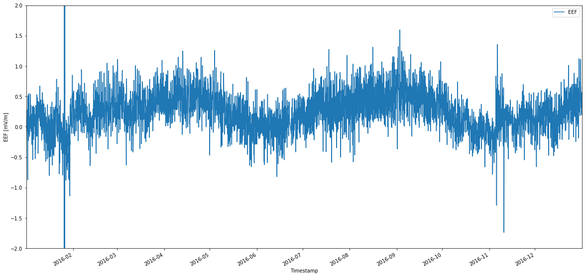
Take a look at the time jumps between entries… Nominally the product should produce one measurement “every dayside equator crossing ±20 minutes”
times = df.index
delta_t_minutes = [t.seconds/60 for t in np.diff(times.to_pydatetime())]
print("Range of time gaps (in minutes) between successive measurements:")
np.unique(np.sort(delta_t_minutes))
Range of time gaps (in minutes) between successive measurements:
array([  46.3       ,   46.4       ,   91.48333333,   91.5       ,
         91.51666667,   91.53333333,   91.55      ,   91.56666667,
         91.58333333,   91.6       ,   91.61666667,   91.63333333,
         91.65      ,   91.66666667,   91.68333333,   91.7       ,
         91.71666667,   91.73333333,   91.75      ,   91.76666667,
         91.78333333,   91.8       ,   91.81666667,   91.83333333,
         91.85      ,   91.86666667,   91.88333333,   91.9       ,
         91.91666667,   91.93333333,   91.95      ,   91.96666667,
         91.98333333,   92.        ,   92.01666667,   92.03333333,
         92.05      ,   92.06666667,   92.08333333,   92.1       ,
         92.11666667,   92.13333333,   92.15      ,   92.16666667,
         92.18333333,   92.2       ,   92.21666667,   92.23333333,
         92.25      ,   92.26666667,   92.28333333,   92.3       ,
         92.31666667,   92.33333333,   92.35      ,   92.36666667,
         92.38333333,   92.4       ,   92.41666667,   92.43333333,
         92.45      ,   92.46666667,   92.48333333,   92.5       ,
         92.51666667,   92.53333333,   92.55      ,   92.56666667,
         92.58333333,   92.6       ,   92.61666667,   92.63333333,
         92.65      ,   92.66666667,   92.68333333,   92.7       ,
         92.71666667,   92.73333333,   92.75      ,   92.76666667,
         92.78333333,   92.8       ,   92.81666667,   92.83333333,
         92.85      ,   92.86666667,   92.9       ,   92.91666667,
         92.95      ,   92.96666667,   92.98333333,   93.        ,
         93.01666667,   93.03333333,   93.05      ,   93.06666667,
         93.08333333,   93.1       ,   93.11666667,   93.15      ,
         93.18333333,   93.2       ,   93.21666667,   93.23333333,
         93.25      ,   93.26666667,   93.28333333,   93.3       ,
         93.33333333,   93.35      ,   93.36666667,   93.38333333,
         93.4       ,   93.41666667,   93.43333333,   93.45      ,
         93.46666667,   93.48333333,   93.5       ,   93.51666667,
         93.53333333,   93.55      ,   93.56666667,   93.58333333,
         93.6       ,   93.61666667,   93.63333333,   93.65      ,
         93.66666667,   93.68333333,   93.7       ,   93.71666667,
         93.73333333,   93.75      ,   93.76666667,   93.78333333,
         93.8       ,   93.81666667,   93.83333333,   93.85      ,
         93.86666667,   93.88333333,   93.9       ,   93.91666667,
         93.93333333,   93.95      ,   93.96666667,   93.98333333,
         94.        ,   94.01666667,   94.03333333,   94.05      ,
         94.06666667,   94.08333333,   94.1       ,   94.11666667,
         94.13333333,   94.15      ,   94.16666667,   94.18333333,
         94.2       ,   94.21666667,   94.23333333,   94.25      ,
         94.26666667,   94.28333333,   94.3       ,   94.31666667,
         94.33333333,   94.35      ,   94.36666667,   94.38333333,
         94.4       ,   94.41666667,   94.43333333,   94.45      ,
         94.46666667,   94.48333333,   94.5       ,   94.51666667,
         94.53333333,   94.55      ,   94.56666667,   94.58333333,
         94.6       ,   94.61666667,   94.63333333,   94.65      ,
         94.66666667,   94.68333333,   94.7       ,   94.71666667,
         94.73333333,   94.75      ,   94.76666667,   94.78333333,
         94.8       ,   94.81666667,   94.83333333,   94.85      ,
         94.86666667,   94.88333333,   94.9       ,   94.91666667,
         94.93333333,   94.95      ,   94.96666667,   94.98333333,
         95.        ,   95.01666667,   95.03333333,   95.05      ,
         95.06666667,   95.08333333,   95.1       ,   95.11666667,
         95.13333333,   95.15      ,   95.16666667,   95.18333333,
         95.2       ,   95.21666667,   95.23333333,   95.25      ,
         95.26666667,   95.28333333,   95.3       ,   95.31666667,
         95.33333333,   95.35      ,   95.36666667,   95.38333333,
         95.4       ,   95.41666667,   95.43333333,   95.45      ,
         95.46666667,   95.48333333,   95.5       ,   95.51666667,
         95.53333333,   95.55      ,   95.56666667,   95.58333333,
         95.6       ,   95.61666667,   95.63333333,   95.65      ,
         95.66666667,   95.68333333,   95.7       ,   95.71666667,
         95.73333333,   95.75      ,   95.76666667,   95.78333333,
         95.8       ,   95.81666667,   95.83333333,   95.85      ,
         95.86666667,   95.88333333,   95.9       ,   95.91666667,
         95.93333333,   95.95      ,   95.96666667,   95.98333333,
         96.        ,   96.05      ,   96.08333333,   96.1       ,
         96.11666667,   96.13333333,   96.15      ,   96.16666667,
         96.18333333,   96.2       ,   96.21666667,   96.23333333,
         96.25      ,   96.26666667,   96.28333333,   96.3       ,
         96.31666667,   96.35      ,   96.38333333,   96.4       ,
         96.41666667,   96.48333333,   96.5       ,   96.51666667,
         96.55      ,   96.56666667,   96.58333333,   96.6       ,
         96.61666667,   96.63333333,   96.65      ,   96.66666667,
         96.68333333,   96.7       ,   96.71666667,   96.73333333,
         96.75      ,   96.76666667,   96.8       ,   96.81666667,
         96.83333333,   96.85      ,   96.86666667,   96.88333333,
         96.9       ,   96.91666667,   96.93333333,   96.95      ,
         96.96666667,   96.98333333,   97.        ,   97.01666667,
         97.06666667,   97.08333333,   97.1       ,   97.11666667,
         97.13333333,   97.15      ,   97.16666667,   97.2       ,
         97.21666667,   97.23333333,   97.25      ,   97.26666667,
         97.28333333,   97.3       ,   97.31666667,   97.33333333,
         97.35      ,   97.36666667,   97.38333333,   97.41666667,
         97.46666667,   97.48333333,   97.5       ,   97.51666667,
         97.53333333,   97.55      ,   97.56666667,   97.58333333,
         97.6       ,   97.61666667,   97.63333333,   97.65      ,
         97.66666667,   97.7       ,   97.73333333,   97.76666667,
         97.78333333,   97.8       ,   97.81666667,   97.83333333,
         97.85      ,   97.86666667,   97.88333333,   97.9       ,
         97.91666667,   97.93333333,   97.96666667,   97.98333333,
         98.        ,   98.01666667,   98.03333333,   98.05      ,
         98.06666667,   98.08333333,   98.1       ,   98.11666667,
        145.23333333,  187.48333333,  187.51666667,  187.56666667,
        187.61666667,  187.68333333,  187.76666667,  187.83333333,
        188.11666667,  188.46666667,  188.83333333,  189.46666667,
        189.48333333,  189.55      ,  189.58333333,  189.61666667,
        189.68333333,  189.93333333,  190.3       ,  190.68333333,
        190.76666667,  191.18333333,  191.2       ,  191.21666667,
        191.26666667,  191.28333333,  191.33333333,  191.36666667,
        191.38333333,  191.45      ,  191.48333333,  191.58333333,
       1421.48333333])
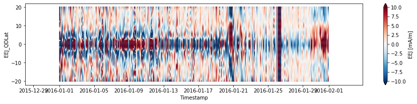
Access the EEJ estimate via xarray instead of pandas
Since the EEJ estimate has both time and latitude dimensions, it is not suited to pandas. Here we load the data as a xarray.Dataset which better handles n-dimensional data.
ds = data.as_xarray()
ds
<xarray.Dataset>
Dimensions:     (EEJ_QDLat: 81, Timestamp: 5508)
Coordinates:
  * Timestamp   (Timestamp) datetime64[ns] 2016-01-01T00:52:23.367156267 ... 2016-12-31T23:20:06.076265574
  * EEJ_QDLat   (EEJ_QDLat) float64 -20.0 -19.5 -19.0 -18.5 ... 19.0 19.5 20.0
Data variables:
    Spacecraft  (Timestamp) object 'B' 'B' 'B' 'B' 'B' ... 'B' 'B' 'B' 'B' 'B'
    Longitude   (Timestamp) float64 113.8 89.98 66.18 ... -105.3 -129.1 -153.0
    Flags       (Timestamp) uint16 0 0 0 0 0 0 0 0 0 0 0 ... 0 0 0 0 0 0 0 0 0 0
    EEJ         (Timestamp, EEJ_QDLat) float64 -73.91 -60.12 ... -7.573 -9.667
    EEF         (Timestamp) float64 -0.4042 -0.1926 -0.1114 ... 0.4747 0.5628
    Latitude    (Timestamp) float64 7.29 7.578 6.948 ... -7.722 -4.006 -0.7652
Attributes:
    Sources:         ['SW_OPER_EEFBTMS_2F_20160101T000000_20160101T235959_020...
    MagneticModels:  []
    RangeFilters:    []
Let’s select a subset (one month) and visualise it:
_ds = ds.sel({"Timestamp": "2016-01"})

fig, ax1 = plt.subplots(nrows=1, figsize=(15,3), sharex=True)
_ds.plot.scatter(x="Timestamp", y="EEJ_QDLat", hue="EEJ", vmax=10, s=1, ax=ax1)
<matplotlib.collections.PathCollection at 0x7f1663704d10>